Quick Start Guide

Introduction

Welcome to easysurv, an R package developed by the Maple Health Group to support basic survival analysis.

The package helps to plot Kaplan-Meier data, assess the proportional hazards assumptions, and estimate & inspect standard parametric survival extrapolations. easysurv can also assist in mixture cure and spline modelling, although these are not explained in detail here.

This guide covers the quick family of functions:

quick_start
quick_KM
quick_PH
quick_fit
quick_to_XL

for easy survival analysis in just a few steps.

Getting Started

# Start from a clean environment
rm(list=ls())

# Attach the easysurv package
library(easysurv)

# Load an easysurv analysis template
quick_start()

quick_start() creates a new .R script in your R environment, pre-loaded with code for survival analysis using the lung dataset from the survival package.

quick_start2() and quick_start3() use different data sets: “bc” from the flexsurv package and simulated phase III breast cancer trial data from the ggsurvfit package, respectively.

The choice of starting data introduces some variations in code, making it beneficial to review all three templates for a comprehensive understanding of the package’s versatility.

Preparing Your Data

Below, we advise some practices to ensure that easysurv can handle your data.

Data Import

easysurv comes pre-loaded with a few data sets borrowed from other packages. One of these is the lung data set from the survival package, which is accessible by calling easy_lung. We’ll store it into surv_data and inspect the first few rows of the data.

# Data Import ------------------------------------------------------------------
surv_data <- easy_lung

# Inspect the first few rows to check it looks as expected.
head(surv_data, 6)

##   inst      time status age sex ph.ecog ph.karno pat.karno meal.cal wt.loss
## 1    3 10.053388      2  74   1       1       90       100     1175      NA
## 2    3 14.948665      2  68   1       0       90        90     1225      15
## 3    3 33.182752      1  56   1       0       90        90       NA      15
## 4    5  6.899384      2  57   1       1       90        60     1150      11
## 5    1 29.010267      2  60   1       0      100        90       NA       0
## 6   12 33.577002      1  74   1       1       50        80      513       0

When importing your own data, there are a number of functions that can be used depending on the file format of the data. These lines of code are available in the script and can be activated as needed.

# Here are some packages & their functions you might use to import your data:
# - haven::read_sas() for SAS (.sas7bdat) files
# - haven::read_dta() for Stata (.dta) files
# - haven::read_sav() for SPSS (.sav) files
# - readxl::read_excel() for Excel (.xls & .xlsx) files
# - readr::read_csv() for .csv files

Data Manipulation

The data needs to be formatted in a certain way for the survival analysis to proceed smoothly. Don’t worry, the requirements are straightforward! The data will need:

A time variable specifying the times to events.
A binary event column specifying whether the event was right-censored (event = 0) or an event (event = 1).
A strata column specifying some way to stratify the events if a comparison is of interest.

Let’s apply these requirements to the easy_lung dataset we imported and stored as surv_data.

# Attach dplyr for data manipulation
library(dplyr)

# Manipulate the data to use with easysurv
surv_data <- surv_data |>
  dplyr::mutate(
    time = time,
    event = status - 1,
    strata = sex
  ) |>
  dplyr::mutate_at("strata", as.factor) |>
  dplyr::as_tibble() |>
  dplyr::select(time, event, strata) # Optional: Just keep variables of interest

We took the following steps:

Left time as is.
Generated event variable by transforming the existing status variable. status was coded as “1” for censoring and “2” for events, but our package (in line with standard survival packages) uses “0” for right-censoring and “1” for events. So we simply subtracted 1 from status.
Generated the strata variable using sex, later converting it to a factor.
Converted the dataset into a “tibble” for easier handling, and removed unnecessary columns using select().

Data Labelling and Inspection

# Check the sample size of each strata
surv_data |> count(strata)

## # A tibble: 2 × 2
##   strata     n
##   <fct>  <int>
## 1 1        138
## 2 2         90

We see that there are 138 instances of the “1” value and 90 instances of the “2” value. Since we’re stratifying by sex, this isn’t very helpful. Let’s then rename these levels as “Male” and “Female”.

We can update other labeling too.

# Assign strata labels in a consistent order with the levels command
levels(surv_data$strata) <- strata_labels <- c("Male", "Female")

# Overwrite any labels impacted by re-coding
attr(surv_data$event, "label") <- "0 = Censored, 1 = Event"

# Define an endpoint label which can be used in plots (if desired)
endpoint_label <- "Overall Survival"

Our data should be ready for survival analysis now, but we want to make sure everything is set up correctly. We can take a look at the top few rows of our tibble, and perform some final sense checks.

# Make sure the data appears as expected.
# A tibble prints the first 10 rows by default
surv_data

## # A tibble: 228 × 3
##     time event strata
##    <dbl> <dbl> <fct> 
##  1 10.1      1 Male  
##  2 14.9      1 Male  
##  3 33.2      0 Male  
##  4  6.90     1 Male  
##  5 29.0      1 Male  
##  6 33.6      0 Male  
##  7 10.2      1 Female
##  8 11.9      1 Female
##  9  7.16     1 Male  
## 10  5.45     1 Male  
## # ℹ 218 more rows

# See sample sizes
surv_data |> count(strata)

## # A tibble: 2 × 2
##   strata     n
##   <fct>  <int>
## 1 Male     138
## 2 Female    90

# See censor/event counts
surv_data |> count(strata, event)

## # A tibble: 4 × 3
##   strata event     n
##   <fct>  <dbl> <int>
## 1 Male       0    26
## 2 Male       1   112
## 3 Female     0    37
## 4 Female     1    53

Quick Workflow Using `easysurv`

Now that our data is properly set up, we can begin with the easysurv analysis.

In this quick workflow, most of the heavy lifting will be done by a set of functions with the quick_ prefix. The first of these is the quick_KM function.

Kaplan Meier analysis

The quick_KM function produces an object with 5 components:

KM_all: A survfit model that includes the whole data set (comparing across strata) using Surv(time, event) ~ as.factor(strata) as the formula.
KM_indiv: A set of survfit models for each individual strata in the data set using Surv(time, event) ~ 1 as the formula.
KM_stepped: A table summarizing the KM survival over time, but presented in a “stepped” manner that is useful for plotting in Excel.
KM_plot: A plot of the Kaplan-Meier curve using the easysurv theme.
KM_summary: Summary information for each of the strata, which includes sample sizes, the number of events, restricted mean survival, median survival and corresponding confidence intervals.

We’ll run this function with our surv_data tibble, providing the names used for the time, event and strata variables, along with a few optional arguments that you can learn about in more detail by typing ?quick_KM into your console.

KM_check <- easysurv::quick_KM(
  data = surv_data,
  time = "time",
  event = "event",
  strata = "strata",

  # Some of the optional arguments for easysurv...
  strata_labels = strata_labels,
  add_time_0 = TRUE,

  # Some of the optional arguments for ggsurvplot...
  title = "Kaplan-Meier Plot",
  subtitle = endpoint_label,
  ylab = endpoint_label,
  xlab = "Months",
  xscale = 1,       # display in months (original)
  break.x.by =  3   # 3 month breaks
)

KM_check

## The quick_KM function has produced the following outputs: 
##  - KM_all
##  - KM_indiv
##  - KM_stepped
##  - KM_plot
##  - KM_summary
##  
##  Assign the output to an object to view it in detail.
##  
##  Below is the KM_summary. The KM_plot has been automatically printed. 
##

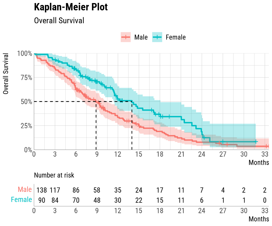
##         group records events    rmean se(rmean)    median   0.95LCL  0.95UCL
## Male     Male     138    112 10.71324 0.7527413  8.870637  6.965092 10.18480
## Female Female      90     53 15.13420 1.1397075 13.995893 11.433265 18.06982
##        Median follow-up
## Male           27.59754
## Female         17.37988

The quick_KM function combines uses of the survival::survfit, easysurv::plot_KM, easysurv::summarise_KM and easysurv::step_KM functions.

To see specific elements of the output, call it by name in double square brackets. For example,

# Not run here
KM_check[["KM_plot"]]

Diagnostic tests

Statistical tests and plots can inform curve fitting approach selection.

The quick_PH() function, where PH = proportional hazards, outputs a list object with five components:

cloglog_plot: A log cumulative hazard plot with the easysurv theme.
coxph_model: A survival::summary.coxPH() object containing statistical test outputs, namely the Cox PH hazard ratio and confidence intervals.
survdiff: A survival::survdiff() object that summarizes a log-rank test, which tests for differences in survival between strata. If p-values are > 0.05, differences are not statistically significant.
coxzph_ph_test: A survival::summary.coxPH() object containing statistical test outputs, namely around whether the data violates the proportional hazards assumption or not.
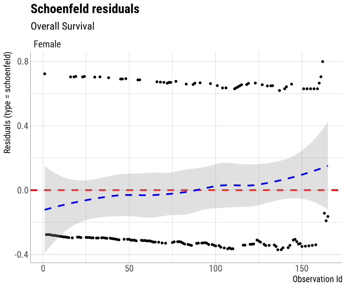
schoenfeld_plot: A Schoenfeld residuals plot in the easysurv theme.

PH_check <- easysurv::quick_PH(
  data = surv_data,
  time = "time",
  event = "event",
  strata = "strata",
  strata_labels = strata_labels, # Optional
  subtitle = endpoint_label # Optional
)

PH_check

## The quick_PH function has produced the following outputs: 
##  - cloglog_plot
##  - coxph_model
##  - survdiff
##  - cox.zph_PH_test
##  - schoenfeld_plot
##  
##  Assign the output to an object to view it in detail. 
##  
## 
## ---- survival::coxph output ----------------------- 
## ---- note: exp(coef) provides Hazard Ratio(s). ---- 
##  
## Call:
## survival::coxph(formula = fit_joint, data = data)
## 
##   n= 228, number of events= 165 
## 
##                 coef exp(coef) se(coef)      z Pr(>|z|)   
## strataFemale -0.5310    0.5880   0.1672 -3.176  0.00149 **
## ---
## Signif. codes:  0 '***' 0.001 '**' 0.01 '*' 0.05 '.' 0.1 ' ' 1
## 
##              exp(coef) exp(-coef) lower .95 upper .95
## strataFemale     0.588      1.701    0.4237     0.816
## 
## Concordance= 0.579  (se = 0.021 )
## Likelihood ratio test= 10.63  on 1 df,   p=0.001
## Wald test            = 10.09  on 1 df,   p=0.001
## Score (logrank) test = 10.33  on 1 df,   p=0.001
## 
## 
##  
##  
##  
## ---- survival::survdiff output -------------------- 
## ---- note: survdiff tests for differences in ------ 
## ---------- survival between strata, using a  ------ 
## ---------- log-rank test.  ------------------------ 
## --------------------------------------------------- 
## ---------- If p-values > 0.05, differences are ---- 
## ---------- not statistically significant. --------- 
##  
## Call:
## survival::survdiff(formula = fit_joint, data = data)
## 
##                 N Observed Expected (O-E)^2/E (O-E)^2/V
## strata=Male   138      112     91.6      4.55      10.3
## strata=Female  90       53     73.4      5.68      10.3
## 
##  Chisq= 10.3  on 1 degrees of freedom, p= 0.001 
## 
##  
##  
##  
## ---- survival::cox.zph output --------------------- 
## ---- note: tests proportional hazards assumption -- 
## --------------------------------------------------- 
## -----------If p-values > 0.05, do not reject ------ 
## -----------PH assumption -------------------------- 
##  
##        chisq df     p
## strata  2.86  1 0.091
## GLOBAL  2.86  1 0.091
## 
##  
##  
## The log cumulative hazard and Schoenfeld residuals plots have been automatically printed.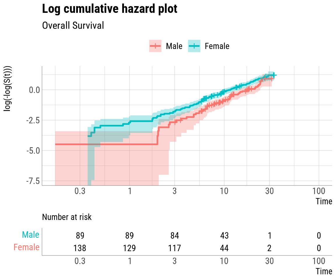

This function combines the use of easysurv::plot_KM() for plotting the log cumulative hazard, survival::coxph() and survival::cox.zph() for fitting a Cox model, survival::survdiff() for testing differences in survival, and easysurv::ggcoxdiagnostics() for producing a Schoenfeld plot.

Fitting Survival Models

Now that we have better statistical awareness of our data, we can fit parametric curves.

easysurv supports 4 different options:

Separate parametric model fitting
Joint parametric model fitting
Mixture cure model fitting
Spline model fitting

In the quick_start() template, we include toggles to decide which of these analyses to perform. This isn’t necessary in all workflows.

## Choose Model Fit Approaches ---------------------------------------------

# After assessing the Kaplan Meier and Proportional Hazards outputs,
# choose a set of analyses to perform.

do_standard <- TRUE # TRUE: run standard parametric model fits (separate)
do_joint <- FALSE # TRUE: run standard parametric model fits (joint)
do_cure <- FALSE # TRUE: run mixture cure model fits
do_splines <- FALSE # TRUE: run spline model fits

We need to specify our distributions of interest. We can choose as many or as few as we want, so long as it’s available as a dist option in flexsurvreg, which is the underlying function of our custom fitting function.

Here, we’re going to fit curves to “Exponential”, “Gamma”, “Generalized Gamma”, “Gompertz”, “log-logistic”, “log-normal” and “Weibull” distributions. With gamma as an exception, these are the distributions recommended by NICE in Technical Support Document (TSD) 14, “Survival analysis: Extrapolating patient data”. Gamma has been included because it has been required by other HTA bodies, including CADTH. The notation for these distributions is defined per flexsurvreg.

dists_global <- c(
  "exp",
  "gamma",
  "gengamma",
  "gompertz",
  "llogis",
  "lnorm",
  "weibull"
)

You can specify the times over which we want to generate and plot extrapolations Here, we’ll use the seq() function to start at time = 0 and go out to 5 times the maximum supplied survival value from the data set. We’ll also specify that between these two times, we want 200 equally spaced time points.

# Times over which to generate/plot extrapolations
times <- seq(
  from = 0,
  to = ceiling(max(surv_data$time) * 5),
  length.out = 200
)

We are now ready to use the quick_fit functions, which consolidate the entire fitting process into one step. There is one function for each type of analysis: quick_fit(), quick_fit_joint(), quick_fit_cure() and quick_fit_splines(). In this case, we will only use quick_fit() since we only want to complete a standard separate parametric fitting. Nevertheless, the process is very similar for the other quick_fit functions and you can get information on each one by typing the name of the function, prefixed with a “?”, in the console.

The script has a set of conditions set up so we don’t need to specifically find the quick_fit functions we want to use and avoid the ones we don’t. We can simply click through the whole “## Model Fitting —-” section.

### Separate fits --------------------------------------------------------------

if (do_standard) {
  dists <- dists_global

  # Toggle line below to see the function help
  # ?quick_fit

  # Fit models
  fit_check <- easysurv::quick_fit(
    data = surv_data,
    time = "time",
    event = "event",
    strata = "strata",
    dists = dists,
    # Optional easysurv arguments
    times = times,
    strata_labels = strata_labels,
    xlab = "Months",
    add_interactive_plots = FALSE
  )
}

To view the output of this object, we can continue to click through the next section, “## See Outputs —-”.

As with the other quick objects, fit_check is a list object with 9 components than can be called individually using double square brackets:

converged: A list of all the successfully converged distributions for each strata.
fits: A survHE::fit.models() output, containing the flexsurv objects for each converged distribution for each strata.
hazard_plots: Smoothed hazard plots for each strata.
hazard_plotly: If the add_interactive_plots argument was set to TRUE. A set of interactive plotly hazard plots, that can accessed in the Viewer panel of RStudio, for each strata.
fit_plots: Plots of the curve extrapolations over the supplied times for each strata.
fit_plotly: If the add_interactive_plots argument was set to TRUE. A set of interactive plotly survival plots, that can accessed in the Viewer panel of RStudio, for each strata.
goodness_of_fit: AIC and BIC outputs, along with their relative ranks for each distribution.
surv_params: The flexsurv parameters for each distribution and strata, along with their variance-covariance matrices.
predicted_fits: Predicted survival proportions over the supplied times for each strata.

For example, we can see a plot of our survival data alongside the curve extrapolations by calling our newly created fit_check and specifying the component of interest using double square brackets.

fit_check[["fit_plots"]][["Male"]]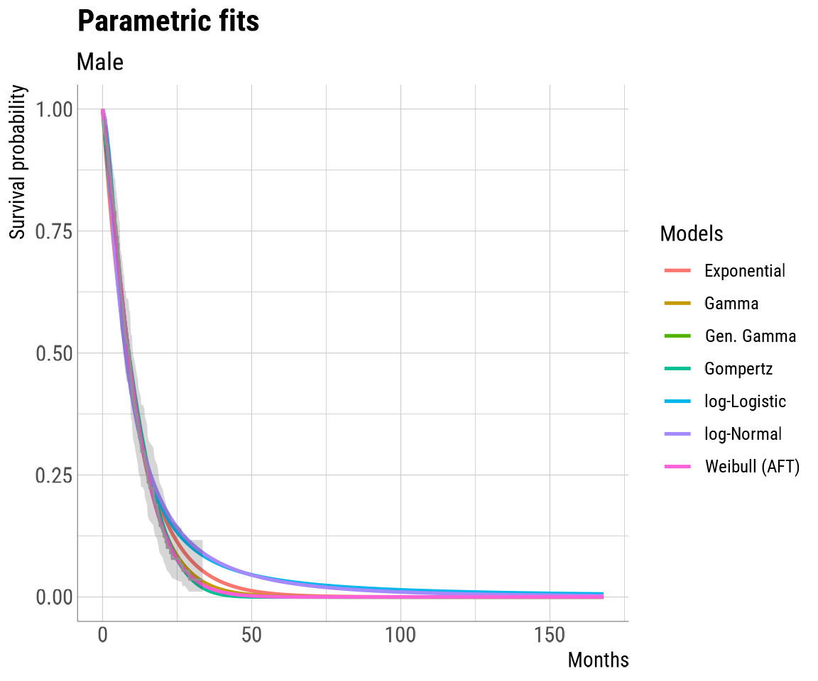

Exporting results to Excel

All of the objects created by the set of quick functions are formatted in such a way that they export easily to Excel. For those who want to export all of these results, we can leverage the openxlsx package. We’ll start by creating a new blank workbook.

## Excel Exports ----------------------------------------------------------------

# Create a new workbook object
wb <- openxlsx::createWorkbook()

We can now use the quick_to_XL function to take each of the objects created by the quick functions and put them in the blank workbook.

# The "quick_to_XL" function prepares easysurv outputs for Excel exporting.
# Note that plots will be reproduced at a different DPI setting for Excel.
# This may make them appear strange in R temporarily.

quick_to_XL(wb = wb, quick_object = KM_check)
quick_to_XL(wb = wb, quick_object = PH_check)

if (do_standard) easysurv::quick_to_XL(wb = wb, quick_object = fit_check)
if (do_joint) easysurv::quick_to_XL(wb = wb, quick_object = fit_check_joint)
if (do_cure) easysurv::quick_to_XL(wb = wb, quick_object = fit_check_cure)
if (do_splines) easysurv::quick_to_XL(wb = wb, quick_object = fit_check_splines)

Lastly, we’ll give this document a name, which is set to be “easysurv output -” along with the date and time. We’ll save the document and open it up.

# Give the workbook a name ending in .xlsx
output_name <- paste0(
  "easysurv output - ",
  format(Sys.time(), "%Y-%m-%d %H.%M"),
  ".xlsx"
)

# Save the workbook - you can choose a directory before this if desired.
openxlsx::saveWorkbook(wb, file = output_name, overwrite = TRUE)

# Open the workbook and assess contents.
openxlsx::openXL(output_name)

Conclusion

And with that, we have a set of standard parametric model outputs in both R and Excel! Look out for future functionality and vignettes and be sure to check out the templates produced by quick_start2() and quick_start3(). If you encounter any bugs or issues, please reach out to the authors.